ArcPad Data Collecting

Introduction
This week we will be going out to the Priory again to collect data using ArcPad. The purpose of this exercise was to introduce us to the use and functions of ArcPad. We had to create a geodatabase from scratch. This database needed to contain features that could be found at the Priory. These features in turn needed to have attributes and have domains.

Methods
The first thing that we did was decided on what we wanted to collect out in the field. My group decided we would map out fallen and dead trees. Both features would be point features. The fallen trees had the attributes of diameter, length, state of decomp, fungal presence,and azimuth. We would use the azimuth and length to generate a line feature showing which way the tree was actually laying. The dead trees had the attributes of diameter, presences of woodpecker, woodpecker use, fungal presence, height and vertical state(leaning or standing). We collected some trees from all over the Priory. Figure 1 shows the final map of our data collection.

Figure 1: Final map of our data collection.

Discussion
The trickiest part of this data collection was getting an accurate measurement of the length of fallen trees and the height of the dead standing trees. This was difficult because we were using a laser range finder to gather the length/height of the trees. This ranger finder works by sending out a laser out at an object and calculating the distance/azimuth of that object. Actually shooting the beam was not difficult. What made it difficult was that there were often branches or bushes in the way of the beam. It would hit these closer objects and not the real target father away, giving us a false reading. Also with the distance we needed to add about 1.7meters to the height attribute of the dead standing trees. This is because when I was shooting the height I was getting a false reading just by standing. I am 5'11" or 1.7m. We needed to add this to the height field because I was shooting the height 1.7m off the ground.

 Below are two maps showing the different attributes on dead standing trees. Figure 2 shows trees grouped by diameter. Figure 3 shows trees grouped by height.

Figure 2: This map shows dead standing trees sorted by diameter

Figure 3: This map shows dead standing trees grouped by height

Below is a map showing the fallen trees and a line feature showing in which direction these trees have actually fallen.

Figure 4: This map shows the fallen trees and the direction they lie

Results
This exercises taught us the importance of thinking and planning ahead about just what you want to collect out in the field. You need to decide what it is you want to collect, what type of feature it is and what types of attributes each of these features need.

HABL Launch

This week we launched the high altitude balloon launch (HABL). This rig is able to reach 100,000 ft above the Earth's surface. We had tested this rig several times during our first two launches with our aerial photography. Figure 1 shows us getting ready to launch our rig into space. Our rig had a video camera and a tracking beacon inside of it. The rig was packed with hand warmers and foam to keep the camera and beacon safe and warm. There was also a parachute attached so that the HABL could return to Earth safely. We did lose the beacon for almost an 1.5. But finally we were able to get a lock on it. The rig had landed in Marshfield, Wisconsin. This is about 78 miles east of Eau Claire. Joe and a couple of other students went out to retrieve the rig. Figure 2 shows the HABL had landed in a 50ft tree. To get it out of the tree, Joe had to climb up and get it.  Figure 3 shows our teacher Joe getting the rig out of the tree that it landed in. 

Figure1

Figure 2: The HABL up in a tree

Figure 3: Joe climbing up to get the HABL

Figure 4: The HABL is safe on the ground.

Below are some still shots from the footage the HABL took on its journey.

Balloon Mapping 2

Balloon Mapping 1

Introduction: 

 Earlier this year we did some preparation work in order to launch a weather balloon to obtain aerial photography of UW-Eau Claire campus. Thanks to this work done a head of time we were prepared to launch our rig attached to the balloon with no problem. It was decided not to use the soda bottle rigs instead we would use the high altitude balloon launch (HABL) rig as a dry run for the real HABL launch later this semester.

Methods:

In order to have a successful launch the class split up into several different groups to complete these tasks. In order to get the rig into the air we had to get the camera rig ready, get the helium tank down to the shed, get the balloon filled, and measure out 400 ft of rope so we would know how far we know the balloon was up in the air. We also had a person whose sole job was to take pictures and anther to take video.

Below Figure 1 shows the helium the tank down to shed so we could fill the balloon up. Down at the shed the used some plastic tubing to fill the balloon up with helium. They used zip ties to make sure seal the balloon close. Figure 2 shows the filling of the balloon. Figure 3 shows that the balloon is almost filled. Someone had to hold on to the balloon while it was being filled. Figure 4 shows the zip ties being used to seal the balloon.

Figure1: The transportation of the helium tank

Figure 2: Filling up the balloon

Figure 3: Balloon almost filled

Figure 4: Zip ties used to close of the balloon

With the balloon being filled, we needed to get the string measured out so we would know how high the balloon was in the air. To do this we unwound a real of string. At every 50ft interval we marked it with a permanent marker.

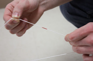
Figure 5: We used Red to mark 50ft and Black to mark 100ft

Figure 6: We used the tiles on the floor, which were one foot long, as a measuring unit to measure out the string

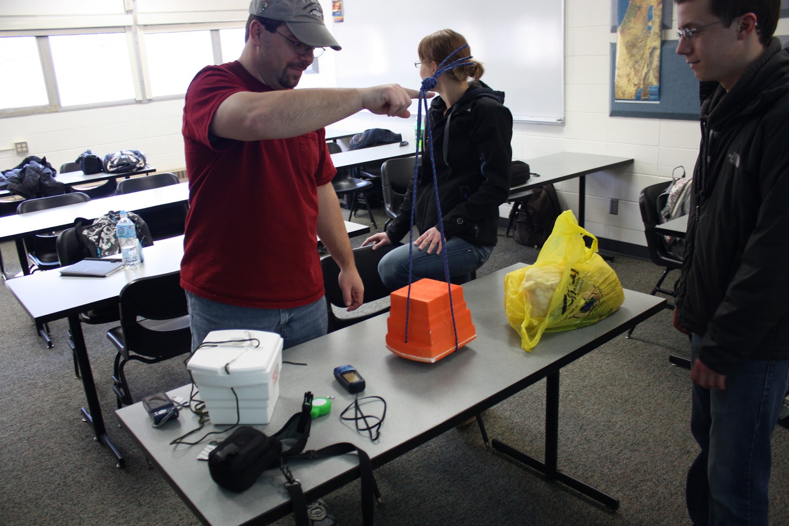
 Earlier this semester we had built two different rigs to hold our camera. However it was decided to use the HABL rig for this launch. By doing this Joe and the rest of the balloon rig engineers would get an idea on how it would react in the real world. Figure 7 shows the two rigs we built earlier this year.  Figure 8 shows the HABL rig that we used for this launch.

Figure 7

Figure 7

Figure 8: the HABL rig. We actually had two rigs built just in case

With all the jobs done we were ready to launch the balloon. We choose to launch the balloon in the center of the green area. UWEC had undergone a large face lift this past year and half. We lost our old Davis center and gained a new one. We are also in the process of building a new education building. With the imagery we would collect with the launch we could get a new aerial view of our new campus. Figure 9 shows us launching the balloon. Figure 10 shows us watching for the 400ft mark that we had mark on the string. 

Figure 9: The launch of the balloon rig

Figure 10: Counting out the feet

After we got the balloon up in the air we walked around the green for awhile. We then took the balloon down so we could switch out the cameras. The first one was a regular camera set on continuous mode. This time we would be using a flipcam that would take video instead of pictures. Figure 11 shows our the flipcam that we used.

Figure 10: The flipcam we used in the second rig

 This time we decided to take the balloon across the foot bridge over the river. We manged to get across the bridge with no problem. The real issue came when we began to reel in the line. The string snapped and the rig fell into the river. The video below shows the string snapping.

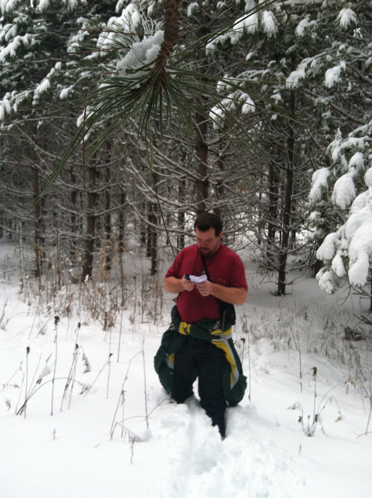
Luckily Joe was able to retrieve the rig from the river. The camera was fine and so was the tracking beacon we placed inside. Figure 11 shows Joe climbing back up to the sidewalk after getting the rig out of the water.

Figure 11: Joe climbed down to the waters edge and used a branch to snag the rig out of the water.

Georeferencing and Mosaic:

Now that we had our images we could georeference them. To georeference an imagine means we take a regular picture and establishes it's location on the Earth. I used ArcMap to georeference the images. I used a reference picture to help me georeference the images. This reference image is already georeferenced and is close to the same resolution of our images, making it ideal for us. When georeferencing you want to get your REMs error as low as possible. Anything around 2 or 1.5 is very good. I tried to get each of my image's REMS error to be around 2 as possible. After the images were georeferenced it was time to mosaic them together. To mosaic an image means to take several smaller images and stitch them together into a larger image. I could have used ArcMap to mosaic the images but instead I used Erdas IMAGINE. It took me about 2-3 hours to get this final image. Figure 12 is my final mosaic over laying the reference image.

Figure 12: Final image

Discussion:

We ran into several problems during this launch and during the post processing. The first problem that we ran into was that it had been very windy that day. Because of the wind our rig was thrown all around and did not take many perpendicular pictures. We need perpendicular images to have a successful mosaic. Figure 13 is an example of an image that is not perpendicular to the ground. While these are interesting to look at they are not useful when mosaicing.

Figure 11: A picture of campus and the River

Another problem that we ran into was the lack of ground points or ground references. Because of all the recent construction we did not have an updated image of what the campus green looks like right now. It is difficult to georeference an image without a good ground references points. It is possible by georeferencing one image very well. Using this image you can then reference the rest of your images by making sure they over lap by at least 60%.

Results:

 In conclusion there are many steps to in making a successful launch for taking aerial photos. It does help to have a lot of people so that these tasks can be split up into more manageable tasks. It is also important to do as much of the prep work before the actual launch date to save yourself headaches and problems. For the actual launch, you want to do it on a day that is clear and has little to no wind. It can take a long time to georeference your images into a good final image. You need a lot of patience and willingness to sometimes through out images to get a perfect final mosaic.

Assignment 8: Final Navigation

Introduction:

Over the past three weeks we have been working on learning different techniques on how to navigate.  We have then taken this knowledge and applied in out in the field. The first week we used the traditional method of using a compass and azimuth to navigate to points out at the Priory. We were also allowed to use a map to help us navigate. The second week we used the GPS to find a new set of points. We were given the coordinates of the points and using the GPS we were to find them without a map. In this final navigation activity, we are to locate all the points that we can in the three hour time period. To spice things up each student will be equipped with a paintball gun.

Study Area:

The navigation course was set up at the Priory which is located about 3 miles south of UW-Eau Claire. The Priory itself is located on a flat plateau surrounded by a wooded area. This wooded area is mainly made up of deciduous trees with a large patch of coniferous to the east of the Priory. The land drops swiftly north and east of the Priory. This year, Wisconsin has experienced a large amount of snow. During all three navigation exercise there was at the very least 6in of snow on the ground. Many times there was deeper especially on the sides of the hills. This made walking around in the woods difficult, most especially when walking up hill.

Methods:

These past few weeks we have gone out to the Priory twice and used a different method each time to navigate around to find points. The two methods that we used were map with compass and GPS. Each method has its own advantages and disadvantages.

Map and Compass

In our first exercise we used the traditional method of using a map and compass to navigate around the Priory. Before actually going out to the Priory, each group made a map that would be used out in the field. Over the map we put a grid. Using this grid we could then plot out where our points were. Also using the grid we were able to get the azimuth from point to point telling us in which direction we needed to be moving in. The map's scale bar gave us an estimate on how far to walk in a certain direction. While this method does work, it is time consuming, you need at least two-three people and does not work well when traveling long distances because it is easy to get of course. Figure 1 shows Stacy and Drew plotting out the points. Figure 2 shows Stacy measuring the azimuth from point to point.

Figure1: Stacy and Drew plotting the points

Figure2: Stacy getting the azimuth

GPS

For the next exercise, we left behind the map and compass moved to a new higher tech method of navigating, the GPS. We were not allowed any map or compass and were only given the coordinates of the points. Using the coordinates, we were to navigate and collect all five points. While this may seem like an easy thing to do, it takes a little bit to get used to using the GPS and knowing which direction you want to walk in. The advantages of this method is that it is highly accurate, simple to use and you only need one person. The disadvantage is that it is dependent on satellites. If you can't connect to a the satellites then your out of luck. Figure 3 shows our GPS and list of coordinates for the points. Also the GPS were keeping a track log so we upload our trail on to the computer to see how well we navigated.  Figure 4 is a map of our course.

Figure3: Garmin etrex GPS and our coordinates to the points

Figure4: Our final map of the track we took out in the field.

Final Outing

On this final outing to the Priory things were going to be a bit different. Instead of collecting points from just one course we were to collect all the points except for the the starting points. At each point we would take a waypoint with the GPS to prove we had been there. Like last time, each student had a GPS with them to record their path. To things more interesting each student was issued a paintball gun. Figures 5-6 show us getting our paintball equipment ready for the field. 

Figure 6: Zach is filling up on of the paintball guns with ammo

Figure6: Paintball equipment laid out and ready to be used.

 There was a five minute grace period so that each team was able to put some distance between each other. My team decided to start with the nearest point and work around in a circle to collect the rest of the points. We were able to stay ahead of other teams for a while but saw some action near point 6. We collected all the points but one.

Assignment 7: Navigation with GPS

Introduction

This week was a continuation of the past several weeks. The class went back out to the Priory to do more navigation exercises. This time around however we were to use a GPS to navigate to our points. We also will not be added by a map. Everyone was assigned a new course to complete. This time my team did course two backward. Every student was issued a Garmin GPS unit. These units served a duel purpose. They were to help us find the points and the other was to record a track log for each student. When we got back to the lab we would use the track logs to create three different maps, a map with just our track log, one with our whole team and one with everyone's track log. The Eau Claire area had just experienced a snow storm earlier that day. There was still some snow flurries when we started out.

Methods

The class met up at the parking lot at the Priory. We were issued a Garmin GPS unit and taught how to record a track log. A track log takes continuous point data that can be used to show a persons path that they took. We were also given the coordinates of a new course. This time my team did course two in reverse. Point 1 is the starting point. From there we went from points 6-2 and then back to 1. We did not have our entire group with us this time. Drew came late after me and Stacy had started the course. Drew caught up with Team 1 and so did the course from 2-6 instead of 6-2. This means his track log will look different from ours so that the team map will look odd.

The Garmin GPS uses UTM eastings and northings to show where on earth a person is. Figure 1 shows a picture of our GPS with it showing the UTM coordinates and a compass. It took me and Stacy a little while to get used to navigating with the GPS units. We ended up going in the wrong direction for a while before we got on the right track. It was a little difficult to figure out in what direction we had to walk in to get the numbers to do what we wanted. At the end of the course we stopped our track logs to complete our paths. We would download the information later back at the lab.

Figure 1: This is our Garmin etrex that we used for this activity. The UTM coordinates are shown at the top of the screen.

In the lab we downloaded the track logs using the DNR Garmin software. We made a point feature class of our track log and put it in a class geodatabase. This way we all had access to each others data to make our maps. We made point features because you can do better analysis using points then with lines. For example you can map out the time field and color the points to show in which direction a person walked. This is what I did in Figure 2. Figure 2 shows a map of my individual track log. The points go from green to yellow to red depicting where I walked when.  Looking at the map you can see it took me and Stacy a little bit to get used to the GPS units. From point 1 to point 6 we started out going in the wrong direction in the beginning. What the map does not show is that we headed down a really steep hill before we figured out we where going in the wrong direction. So it turned out we had to climb back up the hill we just went down.  From point 5 to point 4 we had to navigate around a pond so we could not go in a straight line but had to take a detour.

Figure 2:  A map of my individual track log.

The next map we had to make was a map of our team. Figure 3 shows our team map. Stacy and my tracks line up pretty well. Drew's on the other hand does not. This is because he showed up late and we had already started the course. Drew ended up doing the course with Team 1 who was on course 2 as well. They however were doing the course forward. So Drew's track is going in the opposite direction then ours.

Figure 3: Our team map.

The last map we were to make was one of every students track log. Figure 4 shows a map of every team withe the courses we each did. This time I did not map out the the time attribute of the track logs. Instead to show the different teams I made the points one color so to distinguish the different teams. All the odd numbered teams did their course forward while the even teams went backwards.

Figure 4: A map of every student. The students track logs are color coded depending on which team they were on.

Discussion

I found this activity much easier then using the map and compass. It certainly went a lot faster then the last time when we used the map. When using the map and compass you need to be in a group of a bare minimum of 2 or 3. It is important to have a person to count the paces, one to go ahead of the group and one to hold to compass and instruct the person out front to line up with the azimuth reading. Before heading out you need to plot the points on a map, get the azimuth between the points and the distance between the points. With the GPS units a person could navigate by themselves. All they would need was the coordinates of where they wanted to go. There really is now preparation to do before heading out like there is with the map and compass.

Like I mentioned in the introduction Eau Claire had just got dumped on by a snow storm. We had around 6in of new snow on the ground added to what was already on the ground. For most of the course me and Stacy were walking in snow all the way up to our knees. In some parts of the courses we were walking on the sides of ridges that were very steep and slippery. Me and Stacy ended falling in several places along those ridges. To get to point 5 we had to walk through a large stand of pine trees. These were much easier to walk through because the pine branches caught a lot of the snow, meaning less accumulated on the ground. Figure5-6 show how the deep the snow.

Figure 5: Stacy standing in the snow checking our coordinate

Figure 6: Me standing out in the snow. This was taken in the stand of pine trees. Here we tried to stay under the pines as much as possible because the snow was not as deep as other places like up above.

Results

This week's activity and last week's was to show us difference between traditional navigation(map and compass) vs. GPS navigation.  I believe that it did a very good job of showing the strengths and weaknesses of each method. While the GPS made it easier and faster to navigate, there could be a point when the GPS could not hook up with the satellites.  The traditional navigation does not relay on technology. It can be done anywhere, anytime, in any weather. The downside is that it takes longer to prepare, need to be in group of 2-3 and takes longer than the GPS navigation. Both methods a perfectly viable just depends on the situation you find yourself in when deciding which one to use.






.

Assignment 6: Navigation with Map and Compass

Introduction

This exercise is the implementation of accumulation of skills we have learned in the past few weeks. We are going out the Priory to locate 5 points out in the woods. There were 3 different courses set up. Two teams would be on a course. One team would be going in one direction and the other in the other direction. All of the courses overlapped each other. This was done because there was snow on the ground and we could have followed tracks of the same team on our course to find the point instead of following the compass. With the courses interwoven together, we would have no idea if the tracks led to our points or anther courses points. The weather was overcast. There was snow flurries on and off while we were out there. We  used a map we made last week to plot points that were given to us. Once the points were plotted we then measure the azimuth from point to point so we can navigate once we are out in the field. At each point there was a flag with a hole puncher so we can punch our score card proving that we were at that point.

Methods

Upon arriving at the Priory we went into the building to meet up with our team. Inside we were given points in UTM coordinates. Figure 1 shows our points that we were to find. My team would be doing course 1 backwards. We would not be actually finding point 1 as part of the navigation exercise. Point 1 was used as a starting point. We were then to find points 6-2, in that order.

Figure1: These are the points that we were to find. We used our map to plot the UTM coordinates

We used the map we made last week to plot the points. This map had a grid over the map that was in UTM. I plotted the points and had Stacy and Drew double check my work. Figure 2 shows Stacy and Drew making sure the points were plotted correctly.  Once we were sure that we had our points plotted as accurate as we could get them, we then used a compass to get the azimuth for each point. We measured the azimuth from point 1 to point 6 and so on and so on. We would use these measurements to find our way in the field. Before leaving, we also measured out the distance between the points. We used the scale that was included on our maps and a sheet of paper so we had rough idea of how far we need to travel to find the point. Figure 3 shows us measuring out the azimuth for the points. Figure 4 is a table of our azimuth measurements. When taking the azimuth we did not need to worry about the declination because here in Eau Claire we are basically at zero.

Figure 2: Stacy and Drew checking the plotting of our points

Figure 3: Stacy is measuring out the azimuth using a compass and the map. Drew is recording the measurement

Figure 4: A table of our azimuth and distance to each point

Once we had our map done and had gotten all of our measurements, we went to outside to start the course.  Each person on our team had a specific role to play. Stacy was in charge of the compass. It was his job to make sure we stayed on course with our azimuth reading. Drew was our pacer. Last week we all paced out 100m so we could get our pace count. It was Drew's job to count his paces so we knew how far we had roughly went. My job was to go out in front of the group and stand in a spot on in line with our azimuth so it was possible to stay on course. I would work with Stacy so that we could stay on course. Once I went out a certain distance Drew and Stacy would catch up, Drew counting his steps, and we would start the process over till we found our point. Figure 5 shows me and Drew at the light post that was our starting point.

Figure 5: Me and Drew are all set to start the course.

Once out on the course we quickly figured out that the snow would become a problem. Drew had to adjust his pace count because he took it on a flat surface and he was now walking out in a forest that was covered in snow. We were also having to maneuver through trees both standing and those that had fallen. I could only go so far ahead of the other two because of visibility problems. Figure 6 shows Stacy taking a azimuth reading so we knew which direction to walk in. Figure 7  shows Drew counting out his paces. I am standing at the tree to mark where the path is.  At each point there was a flag and a hole puncher. Each team had a score card that they had to punch to prove that they had been to each point. Figure 8 shows the flag and punch card. Due to time constraints we only made it half way through the course. It took us a long time to get to from point 5 to point 4.

Figure 6: Stacy is using the compass to take an azimuth reading so we knew which direction to travel.

Figure 7: Drew is counting out his paces and I am standing behind a tree marking where he has to walk to

Figure 8: This is one of the flags we had to find. I am punching our card proving that we did indeed get to point 4.

Discussion

We were out on the course for about an hour and a half. Due to time constraints and the fact it was getting dark we only finished half of the course. We located points 6-4. It took us a very long time to get from point 5 to point 4. We were walking through the woods in winter. Which means in Wisconsin there is snow on the ground. The snow could have been as high as a couple of inches in some spots. In others we were walking through a couple of feet. To make matters more interesting the course was set up in such a way that we had to go up and down several hills to get to the points. The snow also caused issues because it hid fallen tree branches and some times whole trees. You did not walk down those hills, it was more like you slid down them. Figure 9 shows one of the hills we had to navigate. If you look up near the top of the picture in the middle, you can see Drew and Stacy coming down the hill.

Figure 9: This picture shows some of the terrain we had to walk through during the course. Stacy and Drew are at the top of the hill coming down to where I am near the bottom.

Due to visibility problems I could only go so far before having to stop and wait for the other two to catch up. These visibility problems were caused by the hilly terrain and the forest itself. Figure 10 shows an example of the low visibility that we had. A lot of the time I could not see Stacy and Drew and they had to shout to me which direction to move in so that i could stay in line with our azimuth reading. We also resorted to hand signals to communicate.

Figure 10: Stacy and Drew are catching up with me. In the woods could not see very clearly very far.

Conclusion

This was a very good exercise. It showed us how to navigate using no technology. All we were allowed to use was a compass and a map. Using the azimuth readings we took and keeping track on how far we had traveled we were able to locate 3 out of 5 points. Given more time I am confident that our team would have found the remaining two points. Next week we will be using GPS units and no maps or compasses to locate a new set of points.