Assignment 4: Distance Azimuth Survey

Introduction

This exercise was learning the different method for surveying. We were to gather different points using distance and azimuth.  After gathering the points, we imported the table into ArcMap and mapped them out on a base map. We gathered data from two different places. The first was a test run to get us familiar with the equipment. We took points in the back of Phillips, the science building at UW Eau Claire. The second time was at Randall Park located two blocks off of Water Street in Eau Claire, Wi. We gathered 10 points at Phillips and 50 at Randall Park.

Methods

Before going out to collect any points using an azimuth it is important to first discover out what your magnetic declination for your location. Magnetic declination is the angle between magnetic north and true north. The declination is positive east of true north and negative west of true north. You need to know what your declination is so you can collect the right azimuth measurement. Once you get your declination you have to adjust you compass or equipment accordingly. We are lucky here in Eau Claire because our declination is 0° 58' W. This is close enough to zero that it makes no difference.

We went out the first time with the entire class. The purpose was for everyone to get used to collecting points using the lasers before we went out on our own in teams of two. We collected points for two statues, an emergency phone, several trees and a building. Stacy and I used a sonic range finder and a compass to gather our points. Figure 1 shows Stacy collecting our point. It happened to be snowing that day so the visibility was a bit bad. 

Figure 1: Stacy is taking a measurement for a point at Phillips Hall.

After collecting the points we went back to the computer lab to enter to our data into the computer. We made an Excel sheet that had five attributes (rows). These were x,y (for the lat, long of the origin point), distance, azimuth and point_number. We imported the table into ArcMap. Using the Bearing Distance to Line we made lines showing our data.

However we ran into some serious problems right away. The first time we tried this, we put in a base map right away. This then set our projection for the layer into a projection. This would not work since we were working in lat long. To find out what our origin’s coordinates are, we planned to use the information tool to pull up those coordinates. But with when the base map was put in first, the layer’s coordinate system was set to a projection, which is in meter not lat long. So the very first thing we learned that we had to do was set the layer’s coordinate system to WGS 1984.  This meant we would be working with lat long not meters even when we brought in the base map.

Now that were working in the right coordinate system, we could get the lat long for our origin point. Our origin point was a tree at the corner of the building that we could see on an aerial map. Those coordinates we plugged into the x,y fields on our table. Using the afore mentioned tool we made our lines. These lines ended up in a residential neighborhood not at Phillips (Figure 2). Figure 3 shows where the lines showed up and where Phillips is. Troubleshooting with the entire class, we found out that our problem was not enough decimal points. At first we used only two but we needed six. When we fixed our x,y coordinates, the lines were in the right place (Figure 4). We used the feature vertices to points to add points at the end our lines showing were the object we were mapping was.

Figure 2: This is where the computer plotted our points the at first. This was when our lat long only had two decimals points.

Figure 3: The red dot is Phillips Hall. This is where the lines should have ended up. The red lines is where the computer plotted our data.

Figure 4: Our final map with the lines in the right place.

For the second part of the exercise, we were to go out in teams of two to map a ¼ hectare plot. Stacy and I decided to go to Randall Park as our study area. We chose this place because it was in easy walking distance from campus. This was important because the night before and continuing into the day, Eau Claire had over 4in of snow. We did not want to travel far with the road conditions.

We decided to map all four corners of the park and collect 12 points from each. It was a bit difficult to find a place for our origin because the sidewalks were covered in snow and we could not quite tell where we were. So for two of the corners we used electrical polls and the other two we uncovered the yellow rumble strips of the crosswalks. We switched off between the two of us as to who was calling out the points and who was recording them. At the park we mapped several different features. These features were trees, benches, picnic tables, a statue, lamp posts, and pavilion polls.

Figure 5: Me taking a measurement at Randall Park

Figure 6: Stacy taking a measurement at Randall Park

After collecting our 50 points which took a little over an hour, we returned to campus. We made an excel sheet out of our data using the attributes from before. We went back to ArcMap and got the coordinates for our four different origin points. This time around we had four different coordinates since we took points at each for corner. Using the Bearing Distance to Line tool we mapped out our data (Figure 7).  To show where our features are we used the Feature Vertices to Points tool to make points out of the end vertices of our lines.

Figure 7: Our final map for Randall Park.

Discussion

The first problem we ran into was when we tried to get our coordinates for our origin points. The very first thing we did when bringing up ArcMap was to add a base map. This base map however was in a projected coordinate system that used meters for units. We needed a coordinate system that used latitude and longitude.After much discussion and experimentation with the whole class, we found out the right sequence of events. Before adding the base map you have to set the Layer's coordinate system to WGS 1984. This way when the base map is brought in, it is automatically projected using a geographical coordinate system which uses lat long as units of measurement.

The second problem we ran into was when we tried to plot our Phillips Hall data the first time around. We were only bringing the Lat Long coordinates out two decimal points. This turned out to be not accurate enough. Our origin point and the place our lines ended up were in the same location according to the data we were feeding our computer (-91.5, 44.79). The entire class was ending up with this problem. Our data was ending up all over the place. Again the class worked together to over come this problem. We found out that our x,y points were not specific enough for the computer to plot them accurately. Our x,y points needed to go out at least six decimal points (-91.499602, 44.796467). This way when we ran our tool the lines ended up at Phillips Hall where they belonged.

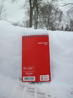
 As I mentioned before the Eau Claire area had experienced a snow storm earliar that day. Thankfully the snow had mainly stopped by the time we went out. This became a problem when just trying to walk around. There was over 5in of snow on the sidewalks (Figure 8).  It also created a problem when we tried to find spots at the corners of the park that could be found on aerial maps. The snow made it had to tell were we actually stood on the sidewalk. As far as we knew we could have been standing on grass or in the street. We chose to use electrical posts as points of origin. Unfortunately these were only at two of the corners. So for the other corners we uncovered the yellow rumble strips at the end of the sidewalks.

Figure 9: A rough estimate of the height of the snow. The notebook is roughly 5.25in tall.

Figure 10: The footprints show where there is a sidewalk that goes through the park.

Figure 11: The yellow rumble strips

We also had some issues when first importing our data. We found out that we made our table wrong. Some of the lines had the wrong origin points and some had the wrong azimuths. These errors were introduced into our data when we copied it over from paper to computer (Figure 12). The table is not the only place where errors could be introduced. Errors may also occur when using any tool in the ArcToolbox. Figure 13 shows what happens when you input the wrong parameters into the tool. I accidentally but the in the distance attribute in the azimuth parameter.  

Figure 12: This map shows our data with an inaccurate table

Figure 13: The lines are facing the wrong way because the parameters were not entered correctly.

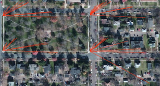
Also we found out that there was a problem with one of points. In the map below you can see that one of the lines shoots far past the park. This happened when trying to collect a measurement for a lamp post. The laser actually picked up the house across the street not the lamp post. The problem was that the lamp post is very skinny and your hand tends to shake when taking a point. The laser went past the post and hit the house. It would have been very nice if we could have had a tripod to use. This way we could have been certain that we got the correct measurement for the feature we wanted.

Figure 14: The line from the bottom right hand corner stretches across the street to a house.

Conclusion

This exercise showed students how one can still collect points without depending on a GPS unit. All one needs is an origin point, some way to measure distance and a compass. Using the distance azimuth methods results with fairly accurate data as long as it is collected correctly.  It also showed us that one has to make accommodations when out in the field depending on what the weather is.